Basics
ModiFinder Basics: Finding Modification Sites
This guide shows you how to use ModiFinder’s core functionality: predicting where structural modifications occur in molecules using MS/MS data.
What is ModiFinder?
ModiFinder compares MS/MS spectra of a known compound and its modified analog to predict the most likely modification sites. It’s particularly useful when you:
Have a known reference compound
Have identified a structurally similar unknown compound
Want to know where the modification occurred
Prerequisites
Before diving into ModiFinder, you might want to familiarize yourself with:
Create Spectrum
The Spectrum modifinder.classes.Spectrum is a class to represent a spectrum, you can create an instance of this object by passing the USI, or from the dictionary of data, or by passing the data for the spectrum fields. check the modifinder.classes.Spectrum for more examples and information.
from modifinder import Spectrum

spectrum = Spectrum("mzspec:GNPS:BERKELEY-LAB:accession:CCMSLIB00010113829")
print(len(spectrum.mz))
36
Create Compound
The Compound modifinder.classes.Compound is the class to represent a Compound, you can create an instance of this object by passing the USI, data in a dictionary or by passing the data for the Compound. Check the modifinder.classes.Compound for documentation and more examples.
from modifinder import Compound

compound = Compound("mzspec:GNPS:BERKELEY-LAB:accession:CCMSLIB00010113829")
print(compound)
Compound(id: CCMSLIB00010113829, name: "methyl 2-amino-4-(2-bromophenyl)-5-oxo-4H-pyrano[3,2-c]chromene-3-carboxylate CollisionEnergy:102040", usi: mzspec:GNPS:GNPS-LIBRARY:accession:CCMSLIB00010113829) with 36 peaks and structure COC(=O)C1=C(N)Oc2c(c(=O)oc3ccccc23)C1c1ccccc1Br
Basic ModiFinder Use
To use ModiFinder modifinder.classes.ModiFinder, start by creating an instance of it. This requires at least two compounds: the target and its known analogs. You can create Modifinder class by using the USIs or using your own data.
Create with USI
You can use ModiFinder in many scenarios but the main one is when you have a known and an unknown compound (with exactly one modification site) and you want to see the likelihood of location the modification. To pass the informations, you can use USI from GNPS. First, Lets Create the Compound objects
from modifinder import ModiFinder, Compound
from matplotlib import pyplot as plt

c1 = "mzspec:GNPS:BERKELEY-LAB:accession:CCMSLIB00010113829"
c2 = "mzspec:GNPS:BERKELEY-LAB:accession:CCMSLIB00010125628"
helpers_array = ['mzspec:GNPS:BERKELEY-LAB:accession:CCMSLIB00010114304']
args = {
    'mz_tolerance': 0.01,
    'ppm_tolerance': 40,
    'ratio_to_base_peak': 0.01,
    'normalize_peaks': True
}
known_compound = Compound(c1, id=c1, **args)
modified_compound = Compound(c2, id=c2, **args)
helpers_compounds = [Compound(h, id=h, **args) for h in helpers_array]
Next, we can define ModiFinder object by passing the Known Compound, ModiFied analog and the helpers to that
mf = ModiFinder(known_compound, modified_compound, helpers=helpers_array, **args)
probs = mf.generate_probabilities()

print("predicted probabilities are: \n", probs)
predicted probabilities are:
 [0.16592098 0.15792845 0.03942338 0.04082704 0.03942338 0.03942338
 0.03942338 0.         0.         0.         0.         0.
 0.         0.         0.         0.         0.         0.
 0.         0.03942338 0.06012586 0.06012586 0.06012586 0.06012586
 0.06012586 0.06012586 0.07745147]
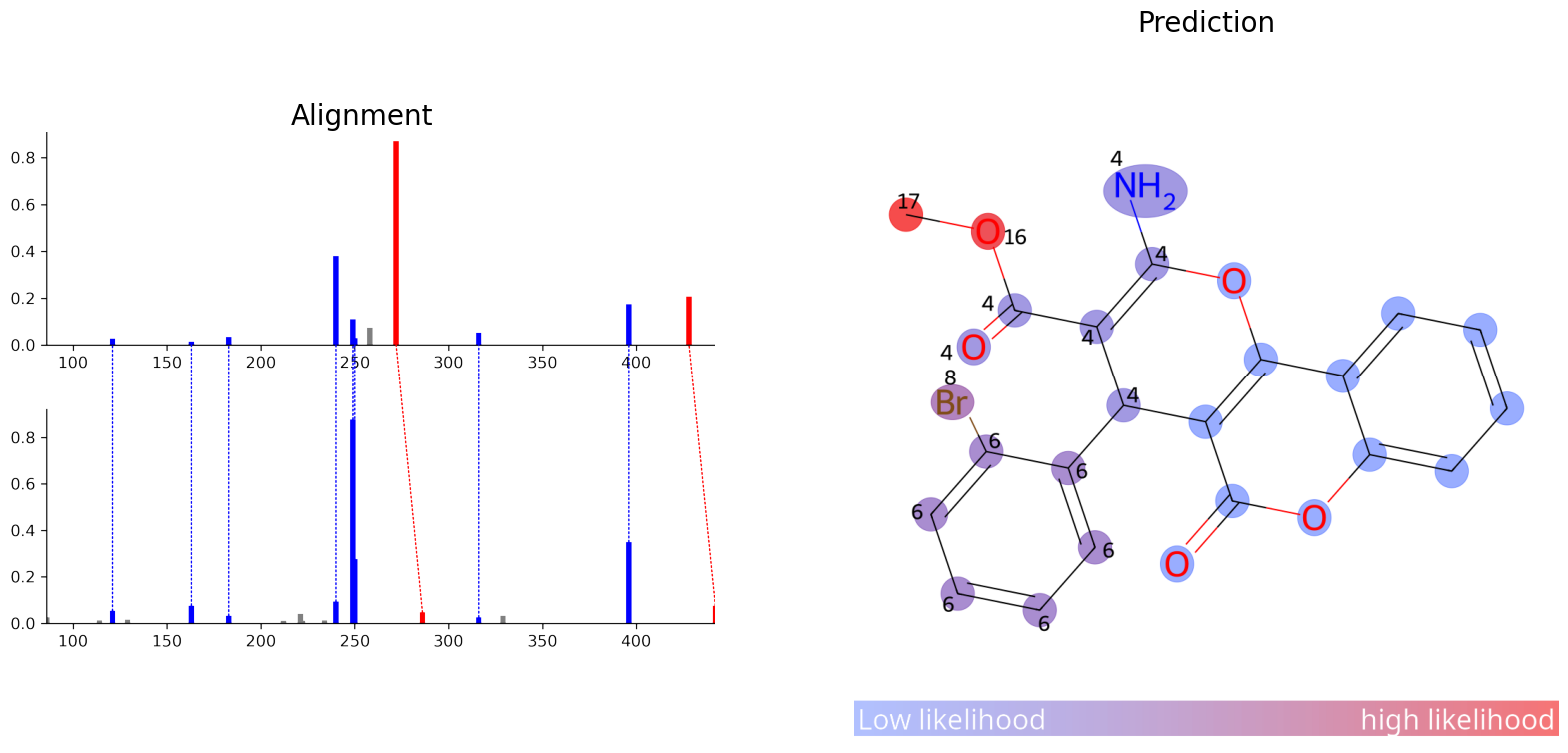
ModiFinder also comes with a lot of visualizing tools, let’s visualize the alignment and the prediction
img_alignment = mf.draw_alignment(known_compound.id, modified_compound.id)

img_prediction = mf.draw_prediction(probs, known_compound.id, show_legend=True, show_labels=True, shrink_labels=True, size=(1000, 1000), annotation_scale = 0.6)

fig, ax = plt.subplots(1, 2, figsize=(20, 10))
ax[0].imshow(img_alignment)
ax[0].set_title('Alignment', fontsize=20)
ax[1].imshow(img_prediction)
ax[1].set_title('Prediction', fontsize=20)

for a in ax:
    a.axis('off')

plt.show()

Oracle
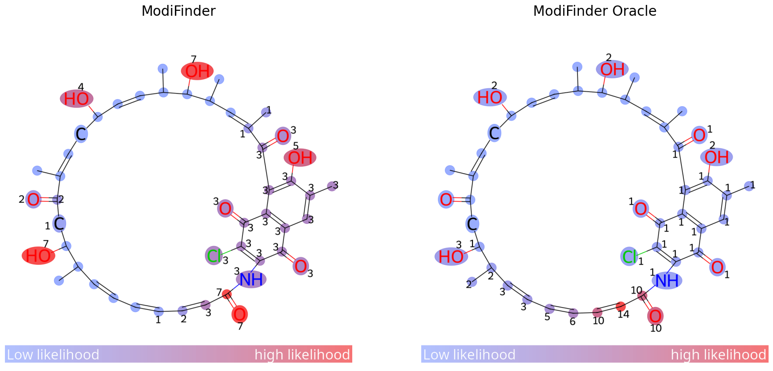
to use ModiFinder in the oracle mode, you can just set the is_known variable of your target compound to True and reannotate the network, this way, the annotation engine will use the structure of the unknown to further refine the peak annotations
oracle_sample_known = Compound("CCMSLIB00011906190", id="known", **args)
oracle_sample_modified = Compound("CCMSLIB00011906105", id="modified", **args)
mf = ModiFinder(oracle_sample_known, oracle_sample_modified, helpers=helpers_array, **args)
probs = mf.generate_probabilities()
img_prediction1 = mf.draw_prediction(probs, oracle_sample_known.id, show_legend=True, show_labels=True, shrink_labels=True, size=(1000, 1000), annotation_scale = 0.6)
mf.network.nodes[oracle_sample_modified.id]["compound"].is_known = True
mf.re_annotate(mf.annotationEngine)
probs = mf.generate_probabilities()
img_prediction2 = mf.draw_prediction(probs, oracle_sample_known.id, show_legend=True, show_labels=True, shrink_labels=True, size=(1000, 1000), annotation_scale = 0.6)
fig, ax = plt.subplots(1, 2, figsize=(20, 10))
ax[0].imshow(img_prediction1)
ax[0].set_title('ModiFinder', fontsize=20)
ax[1].imshow(img_prediction2)
ax[1].set_title('ModiFinder Oracle', fontsize=20)
for a in ax:
    a.axis('off')
plt.show()

Create with your data
You can also create your compounds by passing a dictionary
from modifinder.utilities import visualizer as mf_vis

known_compound_data = {
    "id": "CCMSLIB00010113829",
    "Compound_Name" : "\"methyl 2-amino-4-(2-bromophenyl)-5-oxo-4H-pyrano[3,2-c]chromene-3-carboxylate CollisionEnergy:102040\"" ,
    "Ion_Source" : "LC-ESI",
    "Compound_Source" : "Commercial" ,
    "Instrument" : "Orbitrap" ,
    "PI" : "Trent Northen" ,
    "Data_Collector" : "JGI" ,
    "Adduct" : "M+H" ,
    "Precursor_MZ" : "428.013" ,
    "Charge" : "1" ,
    "Smiles" : "COC(=O)C1=C(N)Oc2c(c(=O)oc3ccccc23)C1c1ccccc1Br",
    "Ion_Mode" : "Positive",
    "ms_level" : "2",
    "peaks" : [[60.998299,2942.000000],[82.425079,2944.000000],[100.039070,16193.000000],[118.427040,3043.000000],[121.018578,3089.000000],[121.028198,88610.000000],[152.897842,2874.000000],[163.038513,46777.000000],[168.043304,5484.000000],[182.943802,109108.000000],[187.409912,3183.000000],[196.038361,3732.000000],[202.218048,2971.000000],[207.029480,3299.000000],[207.976593,4085.000000],[212.033859,24431.000000],[221.989578,4474.000000],[233.956146,5784.000000],[240.028702,1177115.000000],[249.054092,340590.000000],[250.062012,91262.000000],[258.039154,229840.000000],[262.062988,16671.000000],[272.054871,2691841.000000],[275.965454,19609.000000],[280.037537,3552.000000],[281.055145,18616.000000],[288.063934,4550.000000],[289.070587,5006.000000],[299.056152,6172.000000],[316.059662,162469.000000],[317.067596,19549.000000],[328.979919,22114.000000],[377.973846,3657.000000],[395.985809,537614.000000],[428.011810,641369.000000]]
}

modified_compound_data = {
    "id" : "CCMSLIB00010125628",
    "Compound_Name" : "\"ethyl 2-amino-4-(2-bromophenyl)-5-oxo-4H-pyrano[3,2-c]chromene-3-carboxylate CollisionEnergy:205060\"" ,
    "Ion_Source" : "LC-ESI" ,
    "Compound_Source" : "Commercial" ,
    "Instrument" : "Orbitrap" ,
    "PI" : "Trent Northen" ,
    "Data_Collector" : "JGI" ,
    "Adduct" : "M+H" ,
    "Precursor_MZ" : "442.028" ,
    "Charge" : "1" ,
    "Smiles" : "CCOC(=O)C1=C(N)Oc2c(c(=O)oc3ccccc23)C1c1ccccc1Br",
    "ms_level" : "2" ,
    "peaks" : [[66.744087,3088.000000],[68.013557,5761.000000],[68.997673,4342.000000],[84.944817,2668.000000],[86.023949,39517.000000],[87.111252,2685.000000],[88.211983,2617.000000],[91.054718,2792.000000],[96.069580,2500.000000],[106.532509,2811.000000],[114.054657,20689.000000],[121.028481,81112.000000],[129.057541,23604.000000],[140.050171,3201.000000],[142.849548,3238.000000],[155.036545,4860.000000],[163.039078,115792.000000],[168.044922,10549.000000],[182.943878,49352.000000],[191.034134,5956.000000],[194.072769,3414.000000],[205.958740,3058.000000],[207.028503,4013.000000],[207.975830,12770.000000],[212.034348,15917.000000],[214.049545,6682.000000],[221.059967,62232.000000],[222.067261,17084.000000],[233.955292,19126.000000],[234.939468,3125.000000],[240.029068,141213.000000],[249.054565,1321279.000000],[250.062378,417286.000000],[252.948257,4031.000000],[258.038971,6431.000000],[275.964935,6739.000000],[279.358429,2923.000000],[280.038574,5165.000000],[286.036102,2804.000000],[286.070740,71269.000000],[288.065002,4675.000000],[298.048431,3912.000000],[316.059784,39353.000000],[328.980804,50655.000000],[347.603516,3589.000000],[395.986420,526724.000000],[442.028503,115024.000000],[508.895294,3412.000000]]
}

known_compound = Compound(known_compound_data, **args)
modified_compound = Compound(modified_compound_data, **args)
mf = ModiFinder(known_compound, modified_compound, helpers=helpers_array, **args)
probs = mf.generate_probabilities()

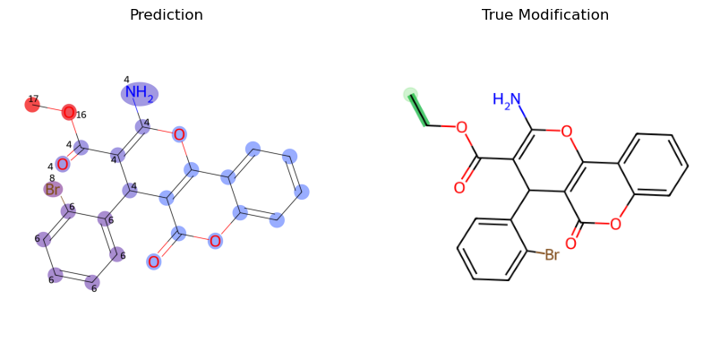
img_prediction = mf.draw_prediction(probs, known_compound.id, show_legend=False, show_labels=True, shrink_labels=True, size=(1000, 1000), annotation_scale = 0.6)

true_modification = mf_vis.draw_modifications(known_compound.structure, modified_compound.structure, show_legend = False,
                                              show_labels=True, shrink_labels=True, modification_only=True)


fig, ax = plt.subplots(1, 2, figsize=(10, 5))
ax[0].imshow(img_prediction)
ax[0].set_title("Prediction")
ax[1].imshow(true_modification)
ax[1].set_title("True Modification")

for a in ax:
    a.axis('off')
plt.show()

Evaluation of the prediction
To assess the accuracy of predictions, several evaluation metrics are available. First, create an instance of the modifinder.engines.evaluation.BasicEvaluationEngine class. Once instantiated, you can input the actual structure of the target compound, its analog, and the prediction into this engine to obtain the evaluation score.
from modifinder import BasicEvaluationEngine

eval_engine = BasicEvaluationEngine()
target_structure = modified_compound.structure
analog_structure = known_compound.structure
eval_score = eval_engine.evaluate_single(analog_structure, target_structure, probs)
print("Evaluation score is: ", round(eval_score, 3))
Evaluation score is: 0.514
If you want to use an evaluation method other than the default, you can just pass that during initialization or when calling the evaluate_single function
eval_engine = BasicEvaluationEngine(default_method="is_max")
target_structure = modified_compound.structure
analog_structure = known_compound.structure
is_max_eval_score = eval_engine.evaluate_single(analog_structure, target_structure, probs)
average_distance_eval_score = eval_engine.evaluate_single(analog_structure, target_structure, probs, evaluation_method="average_distance")
print("IsMax Evaluation score is: ", round(is_max_eval_score, 3), "Average Distance Evaluation score is: ", round(average_distance_eval_score, 3))
IsMax Evaluation score is: 1.0 Average Distance Evaluation score is: 0.514
To learn how you can customize different parts of this process, check the Customization documents